6.2. Unbounded spectral

Definition 6.2.1 (Fourier transform)

The Fourier transform of a function \(u\in L^2\) is the \(L^2\) function

\[ \mathcal{F}[u](k) = \hat{u}(k) = \int_{-\infty}^\infty e^{-ikx}u(x)\, dx, \]

defined for \(k\in \mathbb{R}\), known as the wavenumber.

This is the analysis step. The inverse transform that reconstructs \(u\) from \(\hat{u}\) is called synthesis:

\[ u(x) = \frac{1}{2\pi} \int_{-\infty}^\infty e^{ikx} \hat{u}(k)\, dk. \]

Unbounded grid

If we sample \(u\) on the unbounded grid \(h\mathbb{Z}\), we lose the ability to distinguish all possible wavenumbers, because

\[ e^{i(k+(2\pi/h))x_j} = e^{ikx_j} \cdot e^{i(2\pi/h)(jh)} = e^{ikx_j} \cdot \left( e^{2\pi i} \right)^j = e^{ikx_j}. \]

This effect is called aliasing, and it implies that the wavenumber can be restricted to the domain

\[ -\frac{\pi}{h} \le k < \frac{\pi}{h}. \]

Definition 6.2.2 (Semidiscrete Fourier transform)

A grid function \(v_j\) defined on the unbounded grid \(x_j=jh\), has SFT

\[ \hat{v}(k) = \mathcal{F}_h[v](k) = h \sum_{j=-\infty}^\infty e^{-ikx_j} v_j, \]

defined for \(k\in [-\pi/h,\pi/h)\). The inverse SFT is

\[ v_j = \frac{1}{2\pi} \int_{-\pi/h}^{\pi/h} e^{ikx_j} \hat{v}(k)\, dk. \]

This is actually deeply connected to a standard Fourier series. There, a bounded (periodic) function in space implies discrete wavenumbers, whereas here, discretization in space implies boundedness (periodicity) in wavenumber. Fourier analysis has many such dualities.

Spectral differentiation

The heart of a spectral method is to interpolate the data, differentiate the interpolant, and evaluate on the grid. Interpolation is taken care of by allowing the ISFT to be evaluated at off-grid points:

\[ p(x) = \frac{1}{2\pi} \int_{-\pi/h}^{\pi/h} e^{ikx} \hat{v}(k)\, dk. \]

If we now take the continuous transform of \(p\), we necessarily get

\[\begin{split} \hat{p}(k) = \begin{cases} \hat{v}(k), & |k| \le \pi/h, \\ 0, & \text{otherwise}. \end{cases} \end{split}\]

We call \(p\) the band-limited interpolant of the grid function \(v\). Now we define spectral differentiation of a grid function \(v\) to another grid function \(w\) by

1. Find the band-limited interpolant \(p(x)\) of \(v\).

2. Set \(w_j = p'(x_j)\) for all \(j\).

To find our infinite differentiation matrix, we note that column \(j\) of a matrix can be found by applying it to the vector that has \(1\) in element \(j\) and zero elsewhere. To put this another way, we need to differentiate the following grid function.

Definition 6.2.3 (Grid delta function)

\[\begin{split} \delta_j = \begin{cases} 1, & j=0, \\ 0, & \text{otherwise}. \end{cases} \end{split}\]

Clearly,

\[ \mathcal{F}_h[\delta](k) = h \sum_{j=-\infty}^\infty e^{-ikx_j} \delta_{j} = h, \]

constant for all \(k\) in the wavenumber band. Its BLI is therefore

\[ S_h(x) = \frac{h}{2\pi} \int_{-\pi/h}^{\pi/h} e^{ikx} \, dk = \frac{\sin(\pi x/h)}{\pi x/h}, \]

a sinc function. Thus, column 0 of our infinite differentiation matrix has entries

\[\begin{split} S'_h(x_j) = \begin{cases} 0, & j=0, \\ \dfrac{(-1)^j}{jh}, & j \neq 0. \end{cases} \end{split}\]

This is what we used in the previous section.

Gibbs phenomenon

We can also exploit the obvious fact that

\[ v_j = \sum_{m=-\infty}^\infty v_m \delta_{j-m}. \]

and use linearity to write the band-limited interpolant of \(v\) as

\[ p(x) = \sum_{m=-\infty}^\infty v_m S_h(x-x_m). \]

(Note that shifting \(\delta\) to have center at \(x_m\) does the same thing to the sinc function.)

using Sugar, SpectralMethodsTrefethen
Sugar.get_source(first(methods(p3))) |> last |> print

function p3(h = 1)
    xmax = 10
    fig = Figure()
    x = -xmax:h:xmax                     # computational grid
    xx = -xmax-h/20:h/10:xmax+h/20       # plotting grid
    funs = [
        (x -> float(x == 0), "discrete delta"),
        (x -> float(abs(x) <= 3), "square wave"),
        (x -> max(0, 1 - abs(x) / 3), "tent function")
    ]
    for (plt, (u,label)) in enumerate(funs)
        ax = Axis(
            fig[plt, 1],
            xticksvisible=false, xticklabelsvisible=false,
            yticks=0:1
        )
        (plt==1) && (ax.title = "Convergence of spectral differentiation")
        v = u.(x)
        scatter!(x, v)
        p = [ sum(v[i] * sinc((ξ - x[i]) / h) for i in eachindex(x)) for ξ in xx ]
        lines!(xx, p)
        limits!(ax, -xmax, xmax, -0.5, 1.5)
        text!(-xmax+2, 1.05, text=label)
    end
    return fig
end

p3()

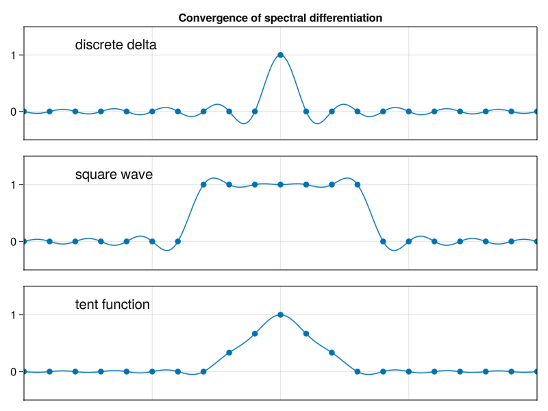
Note in the middle graph above that the BLI is not a great way to approximate a discrete square wave. In fact, it’s worth taking a look at what happens to the square wave as we reduce \(h\) for it:

p3g()

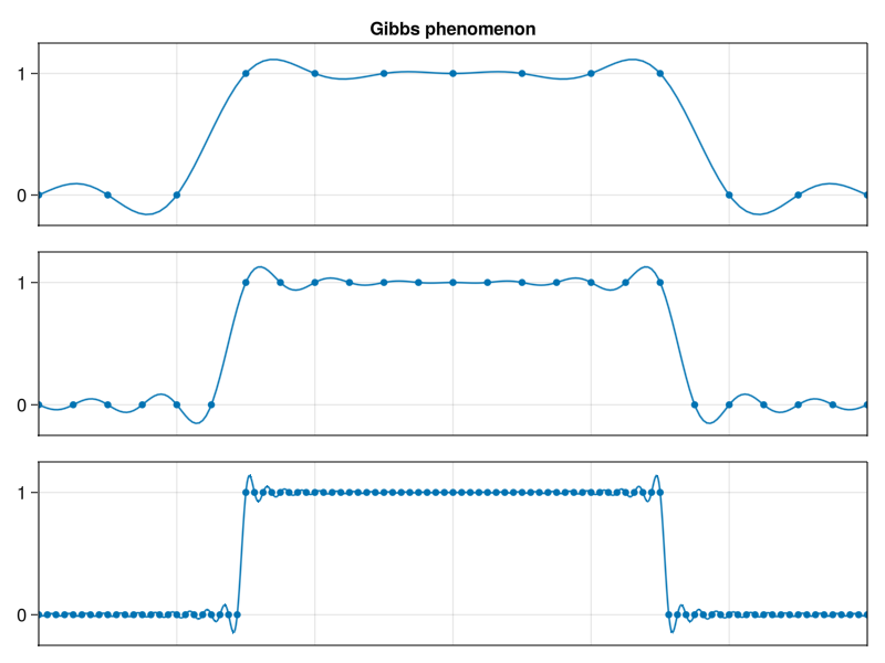
The overshoot in the interpolant gets narrower but not shorter, a fact now known as the Gibbs phenomenon. One point of view is that we get convergence as \(h\to 0 \) in the 2-norm, but not in the \(\infty\)-norm.

Higher derivatives

We can use the same process as above to deduce an infinite differentiation matrix for the second derivative. Column 0 is given by

\[\begin{split} S''_h(x_j) = \begin{cases} -\dfrac{\pi^2}{3h^2}, & j=0, \\ 2\dfrac{(-1)^{j+1}}{j^2h^2}, & j \neq 0. \end{cases} \end{split}\]

Operating in Fourier space

Perhaps the single most attractive feature of the Fourier transform is that differentiation becomes trivial:

\[ \mathcal{F}[u'](k) = ik \,\mathcal{F}[u](k). \]

This gives us an important alternative to the interpolation paradigm above for differentiation of the grid function \(v\) to get \(w\):

1. Set \(\hat{w} = i k\, \hat{v}(k)\).

2. Let \(w = \mathcal{F}_h^{-1}[\hat{w}]\).

Due to all the linearity, this gives an equivalent result, but it is a rather different algorithmic path. Sometimes people reserve the term spectral method for those that operate within wavenumber space like this, while the version that performs all operations within physical space is spectral collocation or (shudder) a pseudospectral method.