6.3. Periodic discrete functions#

In practice, of course, we cannot manipulate infinite grid functions numerically. The next best thing is to assume periodicity in space. We will assume \(u(x)\) is \(2\pi\)-periodic and discretize it over \((0,2\pi]:\)

\[ x_i = ih, \qquad h = \frac{2\pi}{N}, \qquad i=1,\ldots,N. \]

We let \(v_i=u(x_i)\) and, when convenient, allow \(v\) to be extended periodically by assuming \(v_{j+mN}=v_j\) for all integers \(j\) and \(m\).

Caution

We assume throughout that \(N\) is even. The formulas for odd \(N\) are usually different.

Discrete Fourier transform#

Previously, discretization of the function \(u\) on the whole real line caused its transform to be confined to \(k \in (-\pi/h,\pi/h]\). Now, confining the function to \([0,2\pi]\) also causes \(k\) to be discretized. Since \(\pi/h=N/2\), in fact, we have

\[ k \in \left\{ -\frac{N}{2}+1,-\frac{N}{2}+2,\ldots,\frac{N}{2} \right\}. \]

Definition 6.3.1 (Discrete Fourier transform)

The discrete Fourier transform of a discretized, periodic function \(v_j\) is

\[ \mathcal{F}_N[u](k) = \hat{v}_k = h \sum_{j=1}^N e^{-ikx_j}\, v_j, \qquad k = -\tfrac{N}{2}+1,-\frac{N}{2}+2,\ldots,\tfrac{N}{2}. \]

Its inverse is

\[ v_j = \frac{1}{2\pi} \sum_{k=1-(N/2)}^{N/2} e^{ikx_j}\, \hat{v}_k, \qquad j=1,\ldots,N. \]

Sawtooth mode#

The inverse transform formula above has an asymmetry with respect to the mode at

\[ k = \pm \frac{\pi}{h} = \pm \frac{N}{2}. \]

(These are equivalent wavenumbers on the grid, by aliasing.) This is called the sawtooth Fourier mode, because

\[ \exp\left[ i \frac{N}{2} x_j \right] = \exp\left[ i \frac{\pi}{h} (jh) \right] = (-1)^j, \]

i.e., the sawtooth mode toggles between \(1\) and \(-1\) on the grid.

The inverse transform as given above puts all the content in \(k=+N/2\), which is fine for the transform itself, but implies a complex derivative \(\pm (iN/2)\) on the grid that is not in keeping with what the sawtooth itself suggests.

The remedy is to split the content in the sawtooth mode evenly between the equivalent wavenumbers:

\[ v_j = \frac{1}{2\pi} \sideset{}{'}\sum_{k=-N/2}^{N/2} e^{ikx_j}\, \hat{v}_k, \qquad j=1,\ldots,N, \]

where the prime on the sum means to apply a factor of \(1/2\) to the first and last terms. For the transform itself, this makes no change, but at the sawtooth mode, we now differentiate

\[ \frac{1}{2}\left( e^{iNx/2} + e^{-iNx/2} \right) = \cos\left(\frac{Nx}{2}\right), \]

which has derivative zero on the grid.

Before leaving this subject, we point out that the situation above arises only for odd-numbered derivatives. For an even derivative, both forms of the sawtooth yield the same (real) values on the grid, and either form of the transform can be used for band-limited interpolation.

Differentiation matrix#

The band-limited interpolant is now

\[ p(x) = \frac{1}{2\pi} \sideset{}{'}\sum_{k=-N/2}^{N/2} e^{ikx}\, \hat{v}_k, \]

for \(x\in(0,2\pi]\). As always, we can differentiate this interpolant and evaluate it on the grid. But to derive a column of the differentiation matrix, we only need to apply the process to the discrete periodic \(\delta\), where \(d_j=1\) for all \(j=mN\) and \(d_j=0\) otherwise. The resulting \(p\) is the periodic version of the sinc function:

\[ S_N(x) = \frac{\sin(\pi x/h)}{(2\pi/h)\tan(x/2)}, \]

which interpolates the discrete delta while also being \(2\pi\)-periodic. The entries of column 0 in the differentiation matrix \(\bfD_N\) are

\[\begin{split} S'_N(x_j) = \begin{cases} 0, & j=0 (\mod N), \\ \tfrac{1}{2}(-1)^j\cot({jh}/2), & j \neq 0 (\mod N). \end{cases} \end{split}\]

Naturally, column 0 is the same as column \(N\), and the rest of the columns are shifted versions of it. The result is again a circulant matrix.

p4: periodic spectral differentiation#

using LinearAlgebra
N = 24

# Set up grid and differentiation matrix:
h = 2π / N
x = h * (1:N)
entry(k) = k==0 ? 0.0 : 0.5 * (-1)^k * cot(k * h / 2)
D = [ entry(mod(i-j,N)) for i in 1:N, j in 1:N ]

# Differentiation of a hat function:
v = @. max(0, 1 - abs(x - π) / 2)
w = D*v
hat = (;v, w)

# Differentiation of exp(sin(x)):
v = @. exp(sin(x))
vʹ = @. cos(x) * v
w = D*v
error = norm(w - vʹ, Inf)
smooth = (;v, w, error);

using CairoMakie, PyFormattedStrings

fig = Figure()
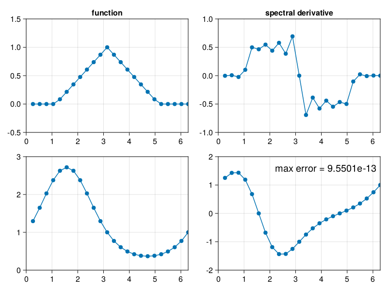
ax = Axis(fig[1, 1], title="function")
scatterlines!(x, hat.v)
limits!(ax, 0, 2π, -0.5, 1.5)
ax = Axis(fig[1, 2], title="spectral derivative")
scatterlines!(x, hat.w)
limits!(ax, 0, 2π, -1, 1)

ax = Axis(fig[2, 1])
scatterlines!(x, smooth.v)
limits!(ax, 0, 2π, 0, 3)
ax = Axis(fig[2, 2])
scatterlines!(x, smooth.w)
limits!(ax, 0, 2π, -2, 2)
text!(2.2, 1.4, text=f"max error = {smooth.error:.5g}", textsize=20)
fig

The differentiation of the nonsmooth function is very poor, but for the smooth case, it’s very accurate.

As before, we can differentiate \(S_N\) twice to get a differentiation matrix for the second derivative. (See textbook.)

FFT#

In the previous section, we observed that one can operate in wavenumber space rather than physical space in order to compute the derivative of a grid function. The same applies in the periodic context:

Set \(\hat{w}_k = i k\, \hat{v}(k)\), except \(\hat{w}_{N/2}=0\).
Let \(w = \mathcal{F}_N^{-1}[\hat{w}]\).

For the \(v\)th derivative, the factor in passing from \(\hat{v}\) to \(\hat{w}\) is \((ik)^\nu\), except it must be set to zero if \(v\) is odd.

This pathway becomes acutely relevant because of the Fast Fourier Transform, credited to Cooley and Tukey in modern times but going back to Gauss. The FFT allows computation of the DFT and IDFT in \(O(N\log N)\) operations, versus the \(O(N^2)\) of a naive DFT implementation as well as for matrix-vector multiplication in physical space. Asymptotically, the FFT pathway should be the fastest by far, although the \(N\) at which it begins to have an advantage is not clear in advance.

In the following code we show how to exploit the fact that a real function has a transform with conjugate symmetry, so that only the first half of the transform needs to be computed explicitly.

p5: repetition of p4 via FFT#

using FFTW 

# real case
function fderiv(v::Vector{T}) where T <: Real
    N = length(v)
    v̂ = rfft(v)
    ŵ = 1im * [0:N/2-1; 0] .* v̂
    return irfft(ŵ, N) 
end

# general case (2x slower)
function fderiv(v)
    N = length(v)
    v̂ = fft(v)
    ŵ = 1im * [0:N/2-1; 0; -N/2+1:-1] .* v̂
    return ifft(ŵ)
end

N = 24

# Set up grid and differentiation matrix:
h = 2π / N
x = h * (1:N)

# Differentiation of a hat function:
v = @. max(0, 1 - abs(x - π) / 2)
w = fderiv(v)
hat = (;v, w)

# Differentiation of exp(sin(x)):
v = @. exp(sin(x))
vʹ = @. cos(x) * v
w = fderiv(v)
error = norm(w - vʹ, Inf)
smooth = (;v, w, error);

using CairoMakie, PyFormattedStrings

fig = Figure()
ax = Axis(fig[1, 1], title="function")
scatterlines!(x, hat.v)
limits!(ax, 0, 2π, -0.5, 1.5)
ax = Axis(fig[1, 2], title="spectral derivative")
scatterlines!(x, hat.w)
limits!(ax, 0, 2π, -1, 1)

ax = Axis(fig[2, 1])
scatterlines!(x, smooth.v)
limits!(ax, 0, 2π, 0, 3)
ax = Axis(fig[2, 2])
scatterlines!(x, smooth.w)
limits!(ax, 0, 2π, -2, 2)
text!(2.2, 1.4, text=f"max error = {smooth.error:.5g}", textsize=20)
fig

Method of lines#

Here is a solution of the variable-coefficient advection PDE

\[ \partial_t u + c(x) \partial_x u = 0, \qquad c(x) = \frac{1}{5} + \sin^2(x-1). \]

Note that the velocity is \(2\pi\)-periodic, which is required for periodic boundary conditions to work as intended.

This function applies the midpoint/leapfrog method in time, with FFT-based spectral differentiation in space:

p6: variable coefficient wave equation#

using FFTW

function p6(⍺ = 1.57)
    # Grid, variable coefficient, and initial data:
    N = 128;  h = 2π / N
    x = h * (1:N)
    t = 0;  Δt = ⍺ / N
    c = @. 0.2 + sin(x - 1)^2
    v = @. exp(-100 * (x - 1) .^ 2)
    vold = @. exp(-100 * (x - 0.2Δt - 1) .^ 2)

    # Time-stepping by leap frog formula:
    tmax = 8
    nsteps = ceil(Int, tmax / Δt)
    Δt = tmax / nsteps
    V = [v fill(NaN, N, nsteps)]
    t = Δt*(0:nsteps)
    for i in 1:nsteps
        w = fderiv(V[:,i])
        V[:,i+1] = vold - 2Δt * c .* w
        vold = V[:,i]
        if norm(V[:,i+1], Inf) > 2.5
            nsteps = i
            break 
        end
    end
    return x,t[1:nsteps+1],V[:,1:nsteps+1]
end

x,t,V = p6(1.57);

using CairoMakie, PyFormattedStrings

fig = Figure()
Axis3(fig[1, 1],
    xticks = MultiplesTicks(5, π, "π"),
    xlabel="x", ylabel="t", zlabel="u", 
    azimuth=4.5, elevation=1.3,
)
gap = max(1,round(Int, 0.15/(t[2]-t[1])) - 1)
surface!(x, t, V, colorrange=(0,1))
[ lines!(x, fill(t[j], length(x)), V[:, j].+.01, color=:ivory) for j in 1:gap:size(V,2) ]
fig

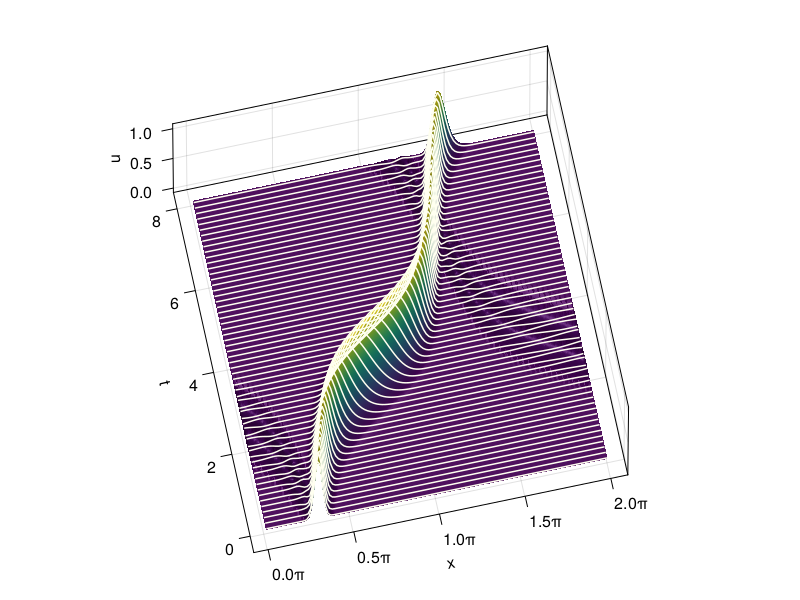
fig = Figure(size=(480,320))
index = Observable(1)
ax = Axis(fig[1, 1],
    xticks = MultiplesTicks(5, π, "π"),
    xlabel="x", ylabel="u"
)
lines!(x, @lift(V[:,$index]))
record(fig, "p6.mp4", 1:4:size(V,2)+1) do i
    index[] = i
    ax.title = f"t = {t[i]:.2f}"
end;

In the simulation above, you can see a small artifact that travels in the wrong direction. The accuracy of this simulation is limited by the second-order time stepping, and even more by the need to estimate the fictitious value \(u(x,-\Delta t)\) that leap frog needs to get started. An automatic, self-starting IVP solver would do much better.

FD and Spectral methods for PDE

Periodic discrete functions

Contents

6.3. Periodic discrete functions#

Discrete Fourier transform#

Sawtooth mode#

Differentiation matrix#

p4: periodic spectral differentiation#

FFT#

p5: repetition of p4 via FFT#

Method of lines#

p6: variable coefficient wave equation#