Barycentric formula
Contents
6.5. Barycentric formula#
When we want to approximate a function on a bounded interval without the benefit of periodicity, the game changes. Attempting to extend the function periodically does permit using Fourier methods, but they will be subject to the Gibbs phenomenon and converge poorly, if at all.
It seems more reasonable instead to interpolate by a polynomial, which makes no assumption about periodicity. It turns out that there are issues of both selecting a well-conditioned polynomial and of evaluating it stably. We begin with the second of these issues.
Derivation#
Recall the Lagrange form of the interpolating polynomial on the nodes \(x_0,x_1,\dots,x_n\):
where
We note that
where \(w_i=1/\Phi'(x_i)\). The constant function 1 is interpolated when all \(y_i=1\), so
which allows us to eliminate \(\Phi\) and write
This is known as the barycentric formula (historically, the second barycentric formula). It’s an odd-looking way to write a polynomial! But it’s been proved to be numerically stable, and it’s efficient, as well.
Usage#
Here is an implementation assuming knowledge of the barycentric weights \(w_j\). Evaluating \(p\) at one point takes only \(O(n)\) flops, regardless of the interpolated function values.
function polyinterp(x, v, w)
    return function(t)
        denom = numer = 0
        for i in eachindex(x)
            if t==x[i]
                return v[i]
            else
                s = w[i] / (t-x[i])
                denom += s
                numer += v[i]*s
            end
        end
        return numer / denom
    end
end
polyinterp (generic function with 1 method)
Computing the weights from the definition takes \(O(n^2)\) operations. Note that a uniform scaling of the weights does not affect the formula, so in practical implementations they are scaled to avoid overflow or underflow in the products.
function polyinterp(x, v)
    C = 4/(maximum(x) - minimum(x))
    weight(i) = 1 / prod(C*(x[i]-x[j]) for j in eachindex(x) if j != i)
    w = weight.(eachindex(x))
    return polyinterp(x,v,w)
end
polyinterp (generic function with 2 methods)
However, the weights are known in closed form in a few cases. For equally spaced nodes in \([-1,1]\), for example,
using Plots

f = x -> sin(exp(x))
x = [0; 3*rand(8); 3]
v = f.(x)
p = polyinterp(x, v)
plot(p, 0, 3, label="polynomial", legend=:bottomleft)
plot!(f, 0,3, color=:black, label="function")
scatter!(x, v, markersize=4, label="data")

Runge phenomenon#
The barycentric formula gives us a stable way to evaluate an interpolating polynomial. However, these polynomials don’t always behave as we would like, particularly on equispaced points.
The Hermite error formula for polynomial interpolation includes a factor \(\Phi(x)\). On equispaced node sets of length \(n+1\), this behaves poorly across the interpolating interval as \(n\to \infty\).
plt = plot(yaxis=(:log,[1e-25,1],"|Φ(x)|"))
t = range(-1,1,1100)
for n in 8:16:56
    x = range(-1,1,n+1)
    Phi = t -> prod(t-x for x in x)
    plot!(t,abs.(Phi.(t)),label="N=$n")
end
plt

In the above, it’s clear that \(\norm{\Phi}_\infty \to 0\) as \(N \to \infty\). However, there is a rapidly widening gap between \(|\Phi|\) near the boundary and near the center. In the next section, we will see that this gap is of size \(2^N\). As it grows, it becomes impossible for machine precision to resolve all of the scales. For \(O(1)\) data, when the error in the middle is \(O(\epsilon_{\text{mach}})\), the error at the boundaries increases beyond \(O(1)\) in order to maintain the gap.
Chebyshev points#
To counteract this effect, we can use interpolation nodes that are more crowded toward the boundaries. Our prime example is the Chebyshev 2nd-kind points,
These points are the abscissas of equally spaced points on the unit circle:
plot([-1,1],[0,0],l=2,aspect_ratio=1,legend=false)
plot!(cos,sin,0,π,l=1)
N = 10
θ = (0:N)*π/N
z = cis.(θ)
x,y = real(z),imag(z)
plot!([x x]',[zero(x) y]',l=(:dash,:black),m=(4,:black))

As we will show in the next section, these points produce a \(|\Phi|\) that is nearly flat across the interval:
plt = plot(yaxis=(:log,[1e-25,1],"|Φ(x)|"))
t = range(-1,1,1100)
for N in 8:16:56
    x = @. cos((0:N)*π/N)
    Phi = t -> prod(t-x for x in x)
    plot!(t,abs.(Phi.(t)),label="N=$N")
end
plt

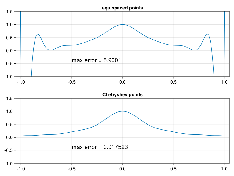
The poor conditioning of equispaced points in polynomial interpolation is known as the Runge phenomenon. It’s typically demonstrated on a very innocuous-looking function, \(1/(1 + 16x^2)\):
p9: polynomial interpolation in equispaced and Chebyshev pts#
include("smij-functions.jl");
using LinearAlgebra

N = 16
data = [
    (@. -1 + 2*(0:N)/N, "equispaced points"),
    (@. cospi((0:N)/N), "Chebyshev points"),
]

xx = -1.01:0.005:1.01
results = []
for (i,(x,label)) in enumerate(data)
    u = @. 1 / (1 + 16 * x^2)
    uu = @. 1 / (1 + 16 * xx^2)
    p = polyinterp(x, u)              # interpolation
    pp = p.(xx)                       # evaluation of interpolant
    error = norm(uu - pp, Inf)
    push!(results, (;x,u,pp,error,label))
end
using CairoMakie, PyFormattedStrings

fig = Figure()
for (i,r) in enumerate(results)
    ax = Axis(fig[i, 1], title=r.label)
    lines!(xx, r.pp)
    scatter!(r.x, r.u)
    limits!(-1.05, 1.05, -1, 1.5)
    text!(-0.5, -0.5, text=f"max error = {r.error:.5g}")
end
fig
It’s also worth noting that the barycentric weights for the 2nd-kind Chebyshev points are simply
We have one last form of polyinterp that assumes the function values are given at the Chebyshev points.
function polyinterp(v)
    N = length(v) - 1
    x = [ cos(j*π/N) for j in 0:N ]
    w = [ float((-1)^j) for j in 0:N ]
    w[[1,end]] .*= 0.5
    return polyinterp(x, v, w)
end
polyinterp (generic function with 3 methods)