6.7. Chebyshev differentiation matrix

Say we are given a grid function \(v\) on the Chebyshev points

\[ x_j = \cos\left( \frac{j\pi}{N} \right), \qquad j=0,\ldots,N. \]

Caution

The definition above orders the Chebyshev points from right to left, which can cause confusion. Note also that there are \(N+1\) of them when we refer to degree \(N\) interpolants.

The Chebyshev spectral collocation scheme is:

1. Let \(p\) be the unique polynomial of degree no more than \(N\) interpolating \(v\) at the \(x_j\).

2. Set \(w_j=p'(x_j)\) for all \(j\).

The process is linear, so there is a matrix \(\bfD_N\) such that

\[ \bfw = \bfD_N \bfv. \]

Note

The restriction to even \(N\) for our Fourier formulas does not apply to the Chebyshev formulas we present.

Unlike the Fourier case, we do not have translation invariance along the Chebyshev grid, so more than one column of \(\bfD_N\) has to be worked out.

Example 6.7.1

For \(N=2\), we have \(x_0=1\), \(x_1=0\), and \(x_2=-1\), and we can write

\[\begin{split} p(x) &= \frac{(x)(x+1)}{(1)(1+1)}v_0 + \frac{(x-1)(x+1)}{(-1)(+1)}v_1 + \frac{(x-1)(x)}{(-1-1)(-1)}v_2 \\ &= \frac{1}{2}(x^2+x)v_0 + (1-x^2)v_1 + \frac{1}{2}(x^2-x)v_2. \end{split}\]

Thus,

\[ p'(x) = \frac{1}{2}(2x+1)v_0 -2x v_1 + \frac{1}{2}(2x-1)v_2, \]

and we get

\[\begin{split} \bfD_2 = \begin{bmatrix} \tfrac{3}{2} & -2 & \tfrac{1}{2} \\ \tfrac{1}{2} & 0 & -\tfrac{1}{2} \\ -\tfrac{1}{2} & 2 & -\tfrac{3}{2} \end{bmatrix}. \end{split}\]

We have seen these rows of numbers occur before, since they arise from finite differences on 3 equally spaced points.

Formulas for the entries of \(\bfD_N\) in the general case are given in the textbook on p. 53. Here is a code that implements them:

using LinearAlgebra
function cheb(N)
    x = [ cos(pi*j/N) for j  in 0:N ]
    c(n) = (n==0) || (n==N) ? 2 : 1
    entry(i,j) = i==j ? 0 : c(i)/c(j) * (-1)^(i+j) / (x[i+1] - x[j+1])
    D = [ entry(i,j) for i in 0:N, j in 0:N ]
    D  = D - diagm(vec(sum(D,dims=2)));    # diagonal entries
    return D, x
end;

The code above does not use the formulas for the diagonal entries. Instead, it uses the negative sum trick, which arises from the fact that the derivative of a constant function is exactly zero in a spectral method, and rewrites the condition \(\sum_j (D_N){ij} = 0\) as an equation for the diagonal term.

Note that the differentiation matrix has the antisymmetry property

\[ (D_N)_{N-i,N-j} = -(D_N)_{i,j}. \]

Otherwise, the matrices do not have much obvious structure:

D, _ = cheb(4)
D

5×5 Matrix{Float64}:
  5.5       -6.82843    2.0          -1.17157    0.5
  1.70711   -0.707107  -1.41421       0.707107  -0.292893
 -0.5        1.41421   -1.11022e-16  -1.41421    0.5
  0.292893  -0.707107   1.41421       0.707107  -1.70711
 -0.5        1.17157   -2.0           6.82843   -5.5

D, _ = cheb(5)
D

6×6 Matrix{Float64}:
  8.5       -10.4721     2.89443   -1.52786    1.10557   -0.5
  2.61803    -1.17082   -2.0        0.894427  -0.618034   0.276393
 -0.723607    2.0       -0.17082   -1.61803    0.894427  -0.381966
  0.381966   -0.894427   1.61803    0.17082   -2.0        0.723607
 -0.276393    0.618034  -0.894427   2.0        1.17082   -2.61803
  0.5        -1.10557    1.52786   -2.89443   10.4721    -8.5

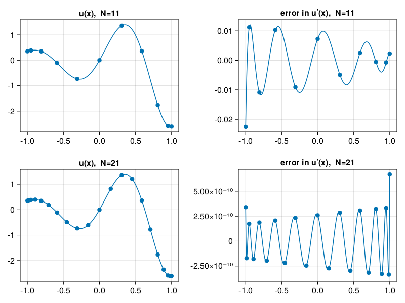
For the analytic, nonperiodic function \(e^x\sin(5x)\), the spectral derivative has about 2 accurate digits at \(N=10\) and 9 at \(N=20\):

p11: Chebyshev differentation of a smooth function

include("smij-functions.jl");

u = x -> exp(x) * sin(5x) 
uʹ = x -> exp(x) * (sin(5x) + 5 * cos(5x))
xx = (-200:200) / 200
vv = @. u.(xx)
results = []
for (i,N) in enumerate([10, 20])
    D, x = cheb(N)
    v = u.(x)
    error = D*v - uʹ.(x)
    ee = polyinterp(x, error).(xx)
    push!(results, (;x,v,error,ee))
end

using CairoMakie
fig = Figure()
for (i,r) in enumerate(results)
    N = length(r.x)
    Axis(fig[i, 1], title="u(x),  N=$N")
    scatter!(r.x, r.v)
    lines!(xx, vv)
    Axis(fig[i, 2], title="error in uʹ(x),  N=$N")
    scatter!(r.x, r.error)
    lines!(xx, r.ee)
end
fig

p12: accuracy of Chebyshev spectral differentiation

The effects of smoothness are illustrated more clearly here:

N = 1:50
# Compute derivatives for various values of N:
data = [ 
    # uʹʹʹ in BV
    (x -> abs(x)^3,  x -> 3x * abs(x), L"|x|^3"), 
    # C-infinity
    (x -> exp(-x^(-2)), x -> 2exp(-x^(-2)) / x^3, L"\exp(-x^{-2})"), 
    # analytic in [-1,1]
    (x -> 1 / (1 + x^2), x -> -2x / (1 + x^2)^2, L"1/(1+x^2)"),
    # polynomial 
    (x -> x^10, x -> 10x^9,  L"x^{10}")
]

results = []
for (i, (fun,deriv,title)) in enumerate(data)
    E = zeros(length(N))
    for (k,N) in enumerate(N)
        D, x = cheb(N)
        E[k] = norm(D*fun.(x) - deriv.(x), Inf)
    end
    push!(results, (;E, title))
end

fig = Figure()
ax = [ Axis(fig[j,i], yscale=log10) for i in 1:2, j in 1:2 ]
for (ax,r) in zip(vec(ax),results)
    ax.title = r.title
    scatterlines!(ax, N, r.E)
end
linkxaxes!(ax...)
linkyaxes!(ax...)
ax[1,1].ylabel = ax[1,2].ylabel = "error"
ax[1,2].xlabel = ax[2,2].xlabel = L"N"
fig

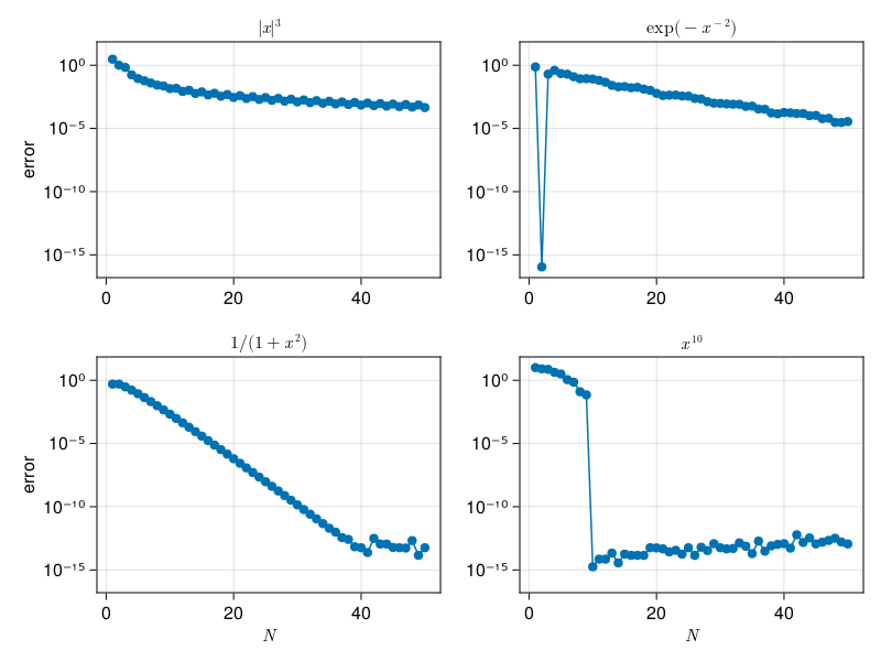
The function \(|x|^3\) has only 2 continuous derivatives, so the convergence is algebraic. Next, \(e^{-x^2}\) is not analytic, and its convergence is between algebraic and exponential. The case \(1/(1+x^2)\) is analytic around the interval, showing spectral convergence, and the function \(x^{10}\) is the polynomial analog of “band-limited.”