Operator splitting
Contents
7.1. Operator splitting#
include("../smim/smij-functions.jl");
A common trick for solving a difficult time-dependent PDE is to split the equation according to
where \(A\) and \(B\) might both include spatial derivatives. Often the motivation is that one of the partial operators is linear or easy to handle for some other reason.
We demonstrate these methods on the Kuramoto–Sivashinsky equation,
With periodic conditions, the last term in the PDE has eigenvalues that are \(O(N^4)\), making the problem quite stiff. However, we can solve in Fourier space via the splitting
which is linear and diagonal, and
which is nonlinear but also nonstiff.
Integrating factor#
Recall that in this case, the splitting is
where \(L\) is linear and responsible for the stiff terms. We multiply this through by \(e^{-tL}\) and define the new variable
so that
For example, if we apply the 2nd-order AB method to this equation, we get
Returning to \(u\) leads to
Or, if we want to use a midpoint RK method, the first stage is
When we translate back to the original variable, and use new stage variables, this becomes
These methods are often applied in Fourier space, where \(L\) is diagonal in most cases. Here again is the IF method, this time applied to the KS equation at second order in time.
N = 140
x, _, _ = trig(N)
x = x .- π
x *= 20/π

m = 1500
Tfin = 100
τ = Tfin/m

u₀ = @. exp(-x^2)

F = plan_rfft(u₀)
F⁻¹ = plan_irfft(F*u₀,N)

ξ = (0:N/2) * π/20
iξ = 1im*[ξ[1:div(N,2)];0]
L = @. ξ^2 - ξ^4
G = û -> -iξ .* (F * (F⁻¹*û).^2 )
#61 (generic function with 1 method)
U = [u₀ zeros(N,m)]
û = F*u₀
E = exp.(τ*L / 2)       # half of the integrating factor
for n = 1:m
    a = τ*G(û)
    b = τ*G(E .* (û + a/2))
    û = @. E*(E*û + b)

    U[:,n+1] = F⁻¹*û       # only needed for plotting
end

using CairoMakie
function animate(name,U)
    index = Observable(1)
    fig = Figure()
    ax = Axis(fig[1,1], xlabel="x", ylabel="u")
    lines!(ax, x, @lift(U[:,$index]))

    record(fig, "$name.mp4", 1:5:m+1) do i
        index[] = i
        ylims!(ax, -2, 2)
    end
    return nothing
end

animate("if2",U)
IMEX methods#
In the event of a linear/nonlinear splitting in the form
a simple idea is to use a hybrid IMEX formula for time-stepping. If the linear part is responsible for the stiffness, then we can simultaneously use an implicit method on the linear part and an explicit one on the nonlinear term. For example, we could combine AM2 (Trapezoid) with AB2 via
Thus, there is only a linear problem to solve for \(u_{n+1}\). We can investigate the absolute stability of this method via the assumptions \(Lu=\lambda u\), \(G(u)=\mu u\), and \(u_k=z^k\), which leads to
For the KS equation, we could set \(\lambda \tau = \alpha\) for \(\alpha<0\) and \(\mu\tau= i\beta\):
using Polynomials
⍺ = range(-31,1,90)
β = range(0,12,90)
zpoly(⍺,β) = Polynomial([1im*β, -2-⍺+3im*β, 2-⍺])
R = [ maximum( abs, roots(zpoly(x,y))) for x in ⍺, y in β ]
contour(⍺, β, R, levels=0.2:0.1:1,
    colorrange=(0.,1.), axis=(xlabel="⍺", ylabel="β"))
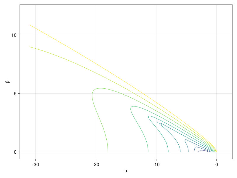
As you can see from the yellow curve above, it appears that we can maintain stability if \(|\beta| < |\alpha|/4\). For the KS equation we might expect \(|\alpha/\beta| = O(N^3)\), so this should not be an issue.
U = [u₀ zeros(N,m)]
û = F*u₀

# one step of BE/Euler to get starting value
G_old = G(û)
û = @. (û + τ*G_old) / (1 - τ*L)
U[:,2] = F⁻¹*û

# TR/AB method
for i in 2:m
    Gu = G(û)
    @. û = ( û + 0.5τ*(L*û + 3Gu - G_old) ) / (1 - 0.5τ*L)
    G_old = Gu
    U[:,i+1] .= F⁻¹*û
end

animate("imex",U)
Split-step integration#
We suppose here that both \(A\) and \(B\) are autonomous (time-invariant). Consider first
Without worrying about it too much, let’s define the exponential of the operator \(A\) via propagation of the initial condition in this problem:
We can do the same for \(B\). The simplest split-step solver of the original PDE is then
If the subproblems are solved exactly, then this method is \(O(\tau)\), i.e., first order. The more symmetric Strang splitting
is second-order in time. It’s normally used by combining the half-step operators in consecutive steps, i.e.,
which is more efficient but does not allow knowing the solution accurately at any time between the start and the end.
We demonstrate split-step on the KS equation by pairing exact advancement of \(e^A\) with a 2nd-order RK method for approximating \(e^B\).
expA = û -> exp.(τ*L) .* û
expA2 = û -> exp.(0.5τ*L) .* û

function expB(û)
    s₁ = τ*G(û)
    return û + τ*G(û + s₁/2)
end;
In order to make the animation easily, we are not merging the half-steps on the \(A\) operator here:
û = F*u₀
U = [u₀ zeros(N,m)]
for n in 1:m
    û = expA2( expB( expA2(û) ) )
    U[:,n+1] = F⁻¹*û
end;

animate("splitstep",U)
Thanks to the Baker–Campbell–Hausdorff formula, there exist split-step methods of any even order. They aren’t often used, though, because they require longer sequences of substeps to advance one full time step, and some of the substep increments are necessarily negative, raising issues with stability (e.g., backward diffusion).
Exponential time differencing#
If we integrate the IF equation over a time step, we get
Returning to the original variable, we get
If we apply, say, a traditional Adams method to solve this equation, we would replace the integrand by a polynomial interpolating it at \(0, -\tau,\ldots.\) However, we might do better approximating the integral via a specialized formula,
where \(P\) interpolates only \(G\) values at the previous time steps. For example, if we use a linear interpolant through \(G_0\) and \(G_{-1}\), we get
where we have used notation that allows \(L\) and \(G\) to be operators as well as scalars. Hence, a 2nd order method is
This type of method is known as exponential time differencing (ETD). There are corresponding formulas based on RK methods, but they are not as easy to describe or derive.
Clearly, we need the ability to evaluate \(e^{\tau L}v\); i.e., to advance the linear part of the PDE one time step. In the KS example, this operator is diagonal in Fourier space, so there is no difficulty, but in other cases, more advanced techniques (e.g., Krylov subspaces) may be used.
More subtly, the method needs a careful implementation to avoid numerical instability. In scalar form, the above formulas are
and it’s clear that we will be up against subtractive cancellation. Cox and Matthews, who first published these methods, suggested using series expansions for small \(\lambda\), which requires diagonalization. However, Kassam and Trefethen showed that one can use contour integrals
as approximated by (wait for it) the trapezoid formula on a closed contour enclosing the eigenvalues.
f₁ = z -> (exp(z) - 1) / z
f₂ = z -> (exp(z) - 1 - z) / z^2
a = zeros(length(L),2)
M = 200
circ = @. cis(2π*(1:M)/M)
for (i,p) in enumerate(τ*L)
    R = max(0.1,abs(0.1*p))  # radius of contour
    z = @. p + R*circ        # points on contour
    dz = @. 1im*R*circ       # dz/dθ

    a[i,1] = τ/M * imag(sum(f₁(z)/(z-p)*dz for (z,dz) in zip(z,dz)))
    a[i,2] = τ^2/M * imag(sum(f₂(z)/(z-p)*dz for (z,dz) in zip(z,dz)))
end

U = [u₀ zeros(N,m)]
û = F*u₀

# one step of BE/Euler to get starting value
G₀ = G(û)
û = @. (û + τ*G₀) / (1 - τ*L)
U[:,2] = F⁻¹*û

E = exp.(τ*L)
for i in 2:m
    G₋₁,G₀ = G₀,G(û)
    û = E.*û + a[:,1].*G₀ + a[:,2].*(G₀-G₋₁)
    U[:,i+1] = F⁻¹*û
end

animate("etd",U)