Chebyshev and the FFT
Contents
6.9. Chebyshev and the FFT#
We will next explore the interactions between three closely related situations:
Chebyshev series, \(x\in [-1,1]\).
Fourier series, \(\theta\in \mathbb{R}\).
Laurent series, \(z\in \mathbb{C}\), \(|z|=1\).
The relationships between these variables are straightforward:
Definition 6.9.1 (Chebyshev polynomial)
The definition alone does not make it clear that \(T_n\) is a polynomial beyond the trivial \(T_0(x)=1\) and \(T_1(x)=x\). But consider that
which proves
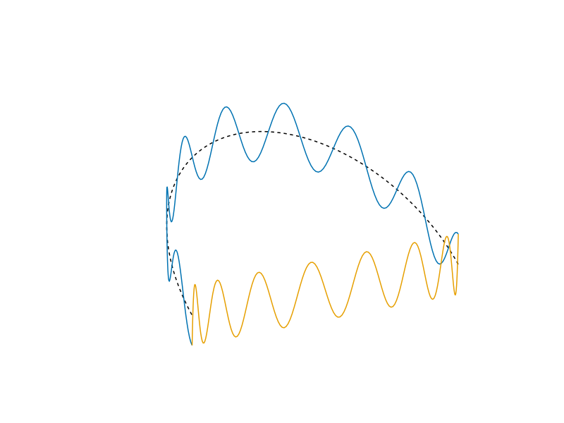
Therefore, each \(T_n\) is a polynomial of degree \(n\) with leading coefficient \(2^{n-1}\). Each Chebyshev polynomial represents even oscillation around the circle but projects down to oscillations pushed out toward the boundaries of \([-1,1]\):
include("smij-functions.jl")
using CairoMakie
fig = Figure(); ax = Axis3(fig[1, 1])
θ = π*(0:200)/200
lines!(cos.(θ),sin.(θ),0*θ,color=:black,linestyle=:dash)
lines!(cos.(θ),sin.(θ),cos.(15θ))
lines!(cos.(θ),0*θ,cos.(15θ))
ax.elevation = 0.2π
ax.azimuth = 1.4π
ax.limits = (-1,1,0,1,-2.5,2.5)
hidedecorations!(ax)
hidespines!(ax)
fig
Chebyshev series#
Any polynomial of degree \(N\) can be written as a combination of the first \(N+1\) Chebyshev polynomials,
Equivalently, we have a Laurent polynomial,
and a trigonometric polynomial,
These are all identical:
when the three variables are related as we have set out. In the limit \(N\to \infty\), each variant becomes an infinite series.
We are interested in using the connections when all the versions of \(p\) interpolate a given grid function. In particular, if \(p\) interpolates a grid function defined at the Chebyshev points in \(x\), then \(\tilde{p}(\theta)\) interpolates a grid function around the unit circle, where each of the interior points defines two values:
using LaTeXStrings
q = π*(0:800)/400
fig = Figure(resolution=(340,340))
ax = Axis(fig[1, 1], aspect=DataAspect())
lines!(cos.(q),sin.(q),color=:black)
lines!([-1,1],[0,0])
θ = π*(0:6)/6
z = cis.(θ)
x = real(z)
[scatterlines!([x,x],[-imag(z),imag(z)],color=:black,linestyle=:dash) for (x,z) in zip(x,z)]
scatter!(x,0*x)
labels = [ latexstring("v_$j") for j in 0:6 ]
text!(Point2(1.06, 0), text=labels[1], align=(:left,:center))
text!(Point2(-1.06, 0), text=labels[7], align=(:right,:center))
text!(x[2:6], sin.(θ[2:6]) .+ 0.08, text=labels[2:6], align=(:center,:bottom) )
text!(x[2:6], -sin.(θ[2:6]) .- 0.05, text=labels[2:6], align=(:center,:top) )

limits!(ax,-1.25, 1.25, -1.25, 1.25)
hidedecorations!(ax)
hidespines!(ax)
fig
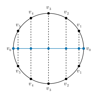
The function \([v_0,v_1,\dots,v_N,v_{N-1},\dots,v_1]\) is even in \(\theta\), which is why a cosine series is sufficient for \(\tilde{p}\). In fact, the DFT of this function gives us the \(a_n\) coefficients directly.
using FFTW
N = 7;
θ = π*(0:N)/N
x = @. cos(θ)
v = @. 2cos(2θ) - 3cos(3θ)
vv = [v; v[N:-1:2]]
fft(vv)/N
14-element Vector{ComplexF64}:
  -3.806478941571965e-16 + 0.0im
   5.075305255429287e-16 + 0.0im
      1.9999999999999996 + 0.0im
     -3.0000000000000004 + 0.0im
   5.075305255429287e-16 + 0.0im
 -1.9032394707859825e-16 + 0.0im
  1.2688263138573217e-16 + 0.0im
                     0.0 + 0.0im
  1.2688263138573217e-16 + 0.0im
 -1.9032394707859825e-16 + 0.0im
   5.075305255429287e-16 + 0.0im
     -3.0000000000000004 + 0.0im
      1.9999999999999996 + 0.0im
   5.075305255429287e-16 + 0.0im
The symmetries in both the data and the transform allow saving space and time by computing only the even (cosine) part by a special syntax. In the case of real data, we use:
FFTW.r2r(v,FFTW.REDFT00) / N
8-element Vector{Float64}:
 -3.806478941571965e-16
  4.440892098500626e-16
  1.9999999999999996
 -3.0
  6.026924990822279e-16
 -2.5376526277146434e-16
  1.2688263138573217e-16
  0.0
Differentiation#
We now have a new algorithmic path for Chebyshev spectral differentiation. By the chain rule,
At \(x=\pm 1\), we have \(\sin(\theta)=0\) and need to apply L’Hôpital’s rule to get
For the second derivative, one finds
except at the endpoints, where special formulas are needed again.
We use the following code to implement Chebyshev differentiation via the FFT.
function chebfft(v)
    # Simple, not optimal. If v is complex, delete "real" commands.
    N = length(v)-1
    N==0 && return [0.0]
    x = [ cos(π*k/N) for k in 0:N ]
    V = [v; v[N:-1:2]]              # transform x -> theta
    U = real(fft(V))
    W = real(ifft(1im*[0:N-1 ;0; 1-N:-1] .* U))
    w = zeros(N+1)
    @. w[2:N] = -W[2:N]/sqrt(1-x[2:N]^2)    # transform theta -> x
    w[1] = sum( n^2 * U[n+1] for n in 0:N-1 )/N + 0.5N*U[N+1];
    w[N+1] = sum( (-1)^(n+1) * n^2 * U[n+1] for n in 0:N-1 )/N + 0.5N*(-1)^(N+1)*U[N+1];
    return w
end
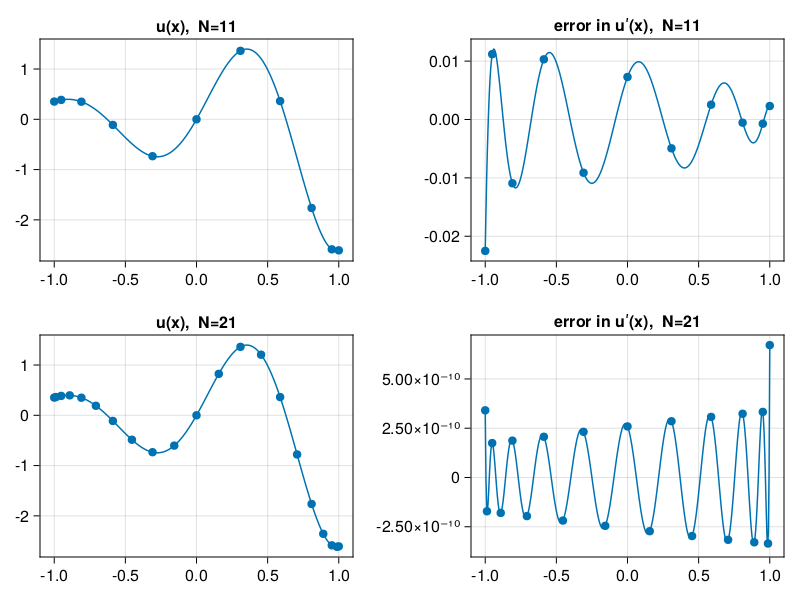
p18: Chebyshev differentiation via FFT (compare p11)#
We reprise a computation done earlier by the differentiation matrix.
u = x -> exp(x) * sin(5x)
uʹ = x -> exp(x) * (sin(5x) + 5 * cos(5x))
xx = (-200:200) / 200
vv = @. u.(xx)
results = []
for (i,N) in enumerate([10, 20])
    _, x = cheb(N)
    v = u.(x)
    error = chebfft(v) - uʹ.(x)
    ee = polyinterp(x, error).(xx)
    push!(results, (;x,v,error,ee))
end
using CairoMakie
fig = Figure()
for (i,r) in enumerate(results)
    N = length(r.x)
    Axis(fig[i, 1], title="u(x),  N=$N")
    scatter!(r.x, r.v)
    lines!(xx, vv)
    Axis(fig[i, 2], title="error in uʹ(x),  N=$N")
    scatter!(r.x, r.error)
    lines!(xx, r.ee)
end
fig
p19: 2nd-order wave eq. on Chebyshev grid (compare p6)#
We can solve the wave equation \(\partial_{tt} u = \partial_{xx} u\) directly as a 2nd-order equation through discretization of the time derivative as a 2nd-order centered difference:
which rearranges to
Even though we have notationally used a differentiation matrix above, we can always replace its application to a vector by the FFT process. We’re being lazy and wasteful here by just applying chebfft twice in a row, rather than properly coding the second derivative directly.
# Time-stepping by leap frog formula:
N = 80
_, x = cheb(N)
Δt = 8 / N^2
v = @. exp(-200 * x^2)
vold = @. exp(-200 * (x - Δt)^2)

tmax = 4
nsteps = ceil(Int, tmax / Δt)
Δt = tmax / nsteps
V = [v fill(NaN, N+1, nsteps)]
t = Δt*(0:nsteps)
for i in 1:nsteps
    w = chebfft(chebfft(V[:,i]))
    w[1] = w[N+1] = 0
    V[:,i+1] = 2V[:,i] - vold + Δt^2 * w
    vold = V[:,i]
    if norm(V[:,i+1], Inf) > 2.5
        nsteps = i
        break
    end
end
using PyFormattedStrings
# Plot results:
fig = Figure()
Axis3(fig[1, 1],
    xticks = MultiplesTicks(5, π, "π"),
    xlabel="x", ylabel="t", zlabel="u", zticks=[-1,1],
    elevation=1.25,
)
gap = max(1,round(Int, 0.075/(t[2]-t[1])) - 1)
surface!(x, t, V, colorrange=(0,1))
[ lines!(x, fill(t[j], length(x)), V[:, j].+.01, color=:ivory) for j in 1:gap:size(V,2) ]
fig
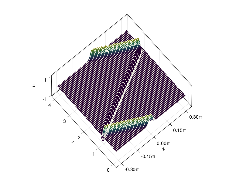
fig = Figure(size=(480,360))
index = Observable(1)
ax = Axis(fig[1, 1],xlabel="x", ylabel="u" )
lines!(x, @lift(V[:,$index]))
record(fig, "p19.mp4", 1:10:size(V,2)+1) do i
    index[] = i
    ax.title = f"t = {t[i]:.2f}"
    limits!(-1,1,-1,1)
end;
p20: 2nd-order wave eq. in 2D via FFT (compare p19)#
The 2D wave equation is analogously solved via
It’s simplest to maintain the unknown \(\bfu\) as a matrix-shaped grid function. Then we can apply chebfft to each column of data for the \(x\) derivatives, and to each row of data for the \(y\) derivatives. To make smooth plots, we also use a grid interpolation function to a finer grid.
# Grid and initial data:
N = 36
x = y = cheb(N)[2]
Δt = 6 / N^2
xx = yy = range(-1,1,81)
nsteps = ceil(Int, 1 / Δt)
Δt = 1 / nsteps

vv = [exp(-40 * ((x - 0.4)^2 + y^2)) for x in x, y in y]
vvold = vv

t = Δt*(0:nsteps)
V = zeros(length(xx),length(yy),nsteps+1)
V[:,:,1] = gridinterp(vv,xx,yy)

# Time-stepping by leap frog formula:
uxx = zeros(N+1, N+1)
uyy = zeros(N+1, N+1)
for n in 1:nsteps
    ii = 2:N
    for i in 2:N
        uxx[i,:] .= chebfft(chebfft(vv[i,:]))
        uyy[:,i] .= chebfft(chebfft(vv[:,i]))
    end
    uxx[[1,N+1],:] .= uyy[[1,N+1],:] .= 0
    uxx[:,[1,N+1]] .= uyy[:,[1,N+1]] .= 0
    vvnew = 2vv - vvold + Δt^2 * (uxx + uyy)
    vvold,vv = vv,vvnew
    V[:,:,n+1] = gridinterp(vv,xx,yy)
end
fig = Figure()
ax = [ Axis3(fig[j,i], zticks=[0,0.5,1]) for i in 1:2, j in 1:2 ]
inc = div(nsteps,3)
for (i,n) in enumerate(1:inc:nsteps+1)
    surface!(ax[i], xx, yy, V[:,:,n], colormap=:blues, colorrange=[-0.3,1.0])
    ax[i].title = f"t = {t[n]:.3f}"
    limits!(ax[i], -1, 1, -1, 1, -0.3, 1)
    ax[i].elevation = π/5
end
fig
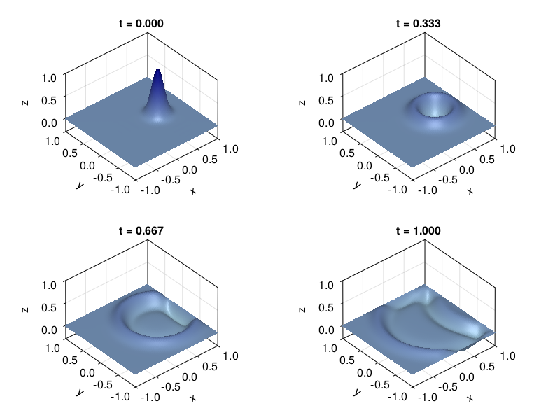
fig = Figure(size=(480,320))
index = Observable(1)
ax = Axis(fig[1, 1], xlabel="x", ylabel="y", aspect=DataAspect())
co = heatmap!(xx, yy, @lift(V[:,:,$index]),
        interpolate=true, colormap=:bluesreds, colorrange=[-0.8,0.8] )
record(fig, "p20.mp4", 1:size(V,3)) do i
    index[] = i
    ax.title = f"t = {t[i]:.2f}"
end;