6.6. Potential theory

Complex analysis is a useful lens through which to view much of approximation theory, particularly when it comes to spectral methods.

The error in polynomial interpolation includes the factor

\[ \Phi(x) = \prod_{j=0}^N (x-x_j), \]

where the \(x_j\) are the interpolation nodes. Taking the log of the modulus yields

\[ \log |\Phi(x)| = \sum_{j=0}^N \log|x-x_j|. \]

This motivates us to define

\[ \phi_N(z) = \frac{1}{N} \sum_{j=0}^N \log|z-x_j|, \]

which is harmonic in the complex plane except at the \(x_j\). There is a compelling physical interpretation of \(\phi_N\) as the electrostatic potential due to point charges in the plane. (A point charge in the plane corresponds to a line of charge in 3D space, which turns the electrostatic force into \(O(|z-x_j|^{-1}\)).)

Things get interesting in the limit \(N\to \infty\). The point charges on \([-1,1]\) become a charge density \(\rho(x)\). If we normalize \(\int_{-1}^1 \rho(x)\, dx\) to be 1, then

\[ \int_a^b \rho(x)\, dx \]

is the fraction of the nodes that lies in the subinterval \([a,b]\). For equispaced points, \(\rho(x)=\tfrac{1}{2}\). For Chebyshev points,

\[ \rho(x) = \frac{1}{\pi\sqrt{1-x^2}}. \]

Key theorem

The potential due to a charge density \(\rho\) is

\[ \phi(z) = \int_{-1}^1 \rho(x)\log|z-x|\, dx. \]

Theorem 6.6.1 (Polynomial potential theory)

Suppose that sets of \(N\) interpolation points \(\{x_j\}\) are given that converge to density function \(\rho(x)\) as \(N\to \infty\). Define the potential \(\phi\) as above, and let

\[ M = \sup_{x\in[-1,1]} \phi(x). \]

Suppose a function \(u\) is analytic throughout the region

\[ \left\{ z\in \mathbb{C}: \phi(z) \le \phi_u \right\}, \]

where \(\phi_u > M\) is a constant, and let \(p_N\) be the polynomial that interpolates \(u\) at the \(\{x_j\}\) for that \(N\). Then there exists a constant \(C>0\) such that

\[ |u(x) - p_N(x)| \le C \exp\left[ -N(\phi_u-M) \right], \]

for all \(x\in[-1,1]\) and all \(N>0\). The same estimate holds, for a different constant \(C\), for any derivative, \(|u^{(d)}(x) - p_N^{(d)}(x)|\).

The theorem promises exponential/geometric convergence over \([-1,1]\) as a function of \(N\), provided \(u\) is analytic throughout some region in \(\mathbb{C}\) that contains the interval.

p10: polynomials and corresponding equipotential curves

using Polynomials

N = 16
data = [
    (@. -1 + 2*(0:N)/N, "equispaced points"),
    (@. cospi((0:N)/N), "Chebyshev points"),
]

xx = -1:0.005:1
xc = -1.4:0.02:1.4
yc = -1.12:0.02:1.12
results = []
for (i,(x,label)) in enumerate(data)
    p = fromroots(x)
    pp = p.(xx)
    pz = [p(x + 1im*y) for x in xc, y in yc]
    push!(results, (;x,pp,pz,label))
end

using CairoMakie

fig = Figure()
levels = 10.0 .^ (-4:0)
for (i,r) in enumerate(results)
    Axis(fig[i, 1], xticks=-1:0.5:1, title=r.label)
    scatter!(r.x, zero(r.x))
    lines!(xx, r.pp)
    
    Axis(fig[i, 2], xticks=-1:0.5:1, title=r.label)
    scatter!(r.x, zero(r.x))
    contour!(xc, yc, abs.(r.pz); levels, color=:black)
    limits!(-1.4, 1.4, -1.12, 1.12)
end
fig

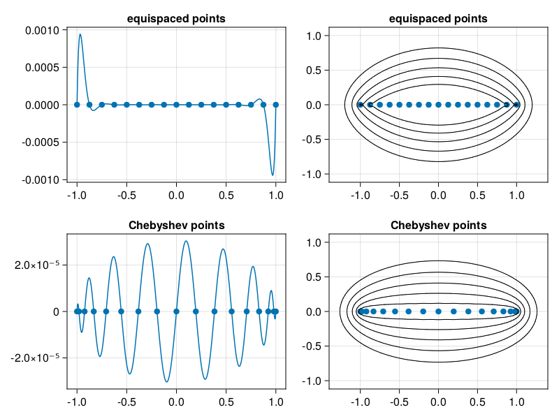
The left column of plots shows \(\Phi(x)\), while the right column shows the level curves of \(\phi\), for both equispaced and Chebyshev points.

Equispaced points

A little elbow grease shows that

\[ \phi(z) = -1 + \frac{1}{2}\text{Re}\left[ (z+1)\log(z+1)-(z-1)\log(z-1) \right]. \]

In particular, \(\phi(0)=-1\) and \(\phi(\pm1) = -1 + \log 2\). Since \(|\Phi(x)|\approx \exp\bigl(N\phi(x)\bigr)\), we find that

\[ \frac{|\Phi(\pm1)|}{|\Phi(0)|} = 2^N. \]

Furthermore, the smallest contour curve of \(\phi\) that contains \([-1,1]\) also contains a significant additional part of the complex plane, requiring “hidden” analyticity for \(u\) beyond the interval itself. The Runge function \(1/(1+16x^2)\), for example, has poles at \(\pm \frac{1}{4}i\), and any equipotential curve that avoids including these will also exclude the ends of the interval.

Chebyshev points

For 2nd-kind Chebyshev points,

\[ \phi(z) = \log \frac{|z + \sqrt{z^2-1}|}{2}. \]

(One has to be careful about how to choose the branch of the square root above.) Remarkably, the interval \([-1,1]\) itself is an equipotential curve for this \(\phi\). More generally, if

\[ z = \frac{1}{2}(r e^{i\theta} + r^{-1} e^{-i\theta}) \]

for \(r > 1\), then \(\phi(z) = \log(r/2)\). This places \(z\) on the ellipse with foci at \(\pm 1\), major axis \(r+r^{-1}\), and minor axis \(r-r^{-1}\). We call this the Bernstein ellipse \(E_r\).

Theorem 6.6.2 (Accuracy of approximation on Chebyshev points)

Suppose \(u\) is analytic on and inside the Bernstein ellipse \(E_r\), let \(d\ge 0\) be an integer, and let \(w_i\) be the \(d\)th Chebyshev spectral derivative of \(u\) on the Chebyshev grid. Then

\[ \left|w_j - u^{(d)}(x_j)\right| = O(r^{-N}), \qquad N\to \infty. \]

We close by noting that the Chebyshev points are not the only ones that allow well-conditioned interpolation. More generally, roots of Jacobi polynomials all have similar density near \(x=\pm 1\), which is the critical property. What distinguishes the Chebyshev case is that the points are known in closed form, and they allow a deep connection to Fourier methods, as we will see.