Chebyshev for BVPs
Contents
6.8. Chebyshev for BVPs#
include("smij-functions.jl");
For the most part, we can drop in a Chebyshev differentiation matrix where we previously used finite differences, but there are some important differences to keep in mind.
1D BVP#
Consider
Unlike FD methods, a reasonable way to get the matrix \(\bfD_{xx}\) is by squaring \(\bfD_x\). (We drop the \(N\) subscript for notational sanity.) Mathematically, both reduce to evaluation of the 2nd derivative of the global polynomial interpolant. For the homogeneous Dirichlet conditions in this example, the numerical solution satisfies \(v_0=v_N=0\), so we can remove both them and the columns of \(\bfD_{xx}\) that they multiply from the linear system \(\bfD_{xx} = \exp(4\bfx)\).
The solution of the linear system produces the grid function \(v\) at Chebyshev points. Unlike FD methods, however, these values also imply a global interpolant over the solution domain. In fact, it would be a crime to use linear interpolation or a cubic spline for off-grid points, as those methods would erase the advantage of spectral accuracy (though you would be unlikely to notice much on a plot of the solution for any smooth method). We use the polyinterp function defined earlier to evaluate the solution anywhere; in principle, we should specialize it to Chebyshev points, for which the barycentric weights are known in closed form, but the performance issue is not meaningful to us for these demonstrations.
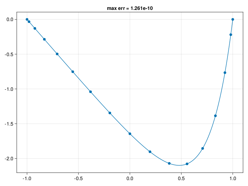
Linear BVP#
p13: solve linear BVP#
N = 16
D, x = cheb(N)
D² = (D^2)[2:N, 2:N]                   # boundary conditions
f = @. exp(4x[2:N])
u = D² \ f                           # Poisson eq. solved here
u = [0; u; 0]
xx = -1:0.01:1
uu = polyinterp(x, u).(xx)      # interpolate grid data
exact = @. (exp(4xx) - sinh(4) * xx - cosh(4)) / 16
err = norm(uu - exact,Inf)
1.2609646660166618e-10
using CairoMakie, PyFormattedStrings

fig = Figure()
Axis( fig[1, 1], title=f"max err = {norm(uu-exact,Inf):.4g}" )
scatter!(x, u)
lines!(xx, uu)
fig
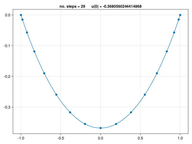
Nonlinear BVP#
For the nonlinear variant
we again derive a nonlinear algebraic system by discretization. Here is a code that uses a fixed-point iteration to approximately solve the nonlinear system:
p14: solve nonlinear BVP#
N = 16
D, x = cheb(N)
D² = (D^2)[2:N, 2:N]
u = zeros(N - 1)
change = 1
it = 0
while change > 1e-15                   # fixed-point iteration
    unew = D² \ exp.(u)
    change = norm(unew - u, Inf)
    u = unew
    it += 1
end
u = [0; u; 0]
xx = -1:0.01:1
uu = polyinterp(x,u).(xx);
fig = Figure()
Axis( fig[1, 1], title="no. steps = $it      u(0) = $(u[N÷2+1])" )
scatter!(x, u)
lines!(xx, uu)
fig
Recall that there are two senses of convergence here: convergence of the iteration as a solution of the discrete equations, and convergence of the discretization to the underlying solution function.
Eigenvalues#
We can also solve the Laplacian eigenvalue problem
We have the exact solutions
p15: solve eigenvalue BVP#
N = 36
D, x = cheb(N)
D² = (D^2)[2:N, 2:N]
λ, V = eigen(D², sortby = (-)∘real)
xx = -1:0.01:1
results = []
for j in 5:5:30                  # plot 6 eigenvectors
    u = [0; V[:, j]; 0]
    uu = polyinterp(x,u).(xx)
    push!(results, (;j,u,uu))
end
using Makie.Colors
fig = Figure()
for (i,r) in enumerate(results)
    ax = Axis(fig[i, 1])
    scatter!(x, r.u, markersize=8)
    line = lines!(xx, r.uu, linealpha=0.5)
    color = line.color[]
    line.color[] = Colors.RGBA(color.r,color.g,color.b,0.4)
    hidespines!(ax); hidedecorations!(ax)
    j = r.j
    text!(-0.4, 0.12, text=f"eig {j} = {λ[j]*4/π^2:#.14g} π^2/4", textsize=20)
    text!(0.7, 0.12, text=f"{4*N/(π*j):.2g} ppw", textsize=20)
end
fig
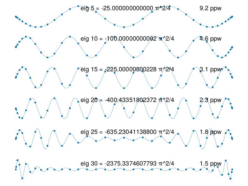
Observe above that the results become increasingly inaccurate as the eigenfunction wavenumber increases. The resolution of a method is often expressed in terms of points per wavelength (PPW), which is the wavelength divided by the grid spacing. As a reference, in Fourier methods the highest wavenumber that can be resolved is \(k=N/2\), and the PPW in this case is
Thus, 2 PPW is the bare minimum for a Fourier spectral method.
For a Chebyshev method, the points are coarsest in the center of the grid, where the node density is \(1/\pi\). This compares to an equispaced node density (on \([-1,1]\)) of \(1/2\), so we lose a factor of \(\pi/2\) in resolution at the center by comparison. It’s therefore reasonable to state that Chebyshev methods have a \(\pi\) PPW minimum resolution requirement.
In the example above, the wavelength of the \(n\)th mode is \(4/n\). Compared to \(h=\pi/N\) at the center, the effective PPW is therefore \(4N/(n\pi)\) at mode \(n\). The figure shows that about 7 digits are correct at PPW 3.1, but the accuracy falls off quickly beyond that.
2D Poisson#
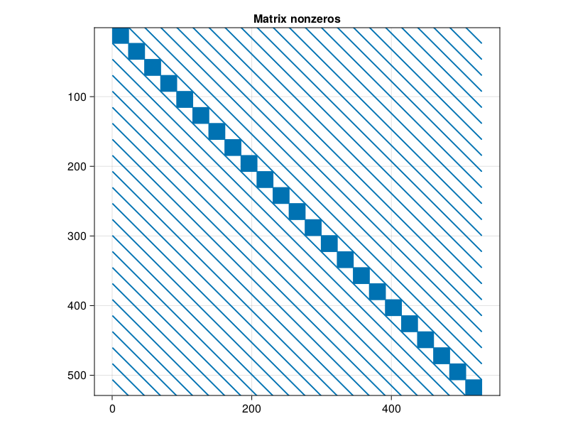
For problems over a rectangle, we can use Kronecker products on a tensor product of Chebyshev grids. The resulting discrete approximation to, say, the Laplacian operator is less sparse than we see with finite differences, the idea is that a much smaller matrix will suffice for equivalent accuracy. If the matrix is truly too large to handle with dense linear algebra, then one can turn to iterative methods with a fast evaluation alternative to be presented in the next section.
One new wrinkle in 2D is that the interpolant must also be evaluated in a tensor-product fashion. For example, suppose a grid function has \(U_{ij}\) given at all \((x_i,y_j)\) for independent Chebyshev grids in \(x\) and \(y\). To evaluate the interpolant at \((\xi,\eta)\), we first evaluate 1D interpolants at \((\xi,y_j)\) for all \(j\), and then do one more 1D evaluation at \((\xi,\eta)\). This can be visualized as collapsing each column of data down to the point \(\xi\), then collapsing the remaining row to a single point. In practice we can do this reasonably efficiently on a grid of \((\xi,\eta)\) values, and we implement that as gridinterp.
function gridinterp(V,xx,yy)
    M,N = size(V) .- 1
    Vx = zeros(length(xx), N+1)
    for j in axes(V,2)
        Vx[:,j] = polyinterp(V[:,j]).(xx)
    end
    VV = zeros(length(xx),length(yy))
    for i in axes(Vx,1)
        VV[i,:] = polyinterp(Vx[i,:]).(yy)
    end
    return VV
end;
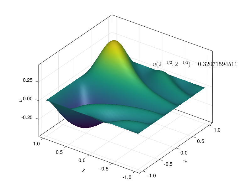
Here is a solution of \(\Delta u = 10\sin(8x(y-1))\) over \([-1,1]^2\) with homogeneous Dirichlet conditions:
p16: Poisson eq. on [-1,1]×[-1,1] with \(u=0\) on boundary#
N = 24
# Set up grids and tensor product Laplacian and solve for u:
⊗ = kron
D, x = D, y = cheb(N)
F = [ 10sin(8x * (y - 1)) for x in x[2:N], y in y[2:N] ]
D² = (D^2)[2:N, 2:N]
L = I(N-1) ⊗ D² + D² ⊗ I(N-1)                     # Laplacian

u = L \ vec(F)           # solve problem

# Reshape long 1D results onto 2D grid (flipping orientation):
U = zeros(N+1, N+1)
U[2:N, 2:N] = reshape(u, N-1, N-1)
value = U[N÷4 + 1, N÷4 + 1]

# Interpolate to finer grid:
xx = yy = -1:0.04:1
UU = gridinterp(U,xx,yy);
using SparseArrays
fig = Figure()
Axis(fig[1, 1], title="Matrix nonzeros", aspect=DataAspect())
row,col,_ = findnz(sparse(L))
scatter!(row, col, markersize=3)
ylims!((N-1)^2, 1)
fig
using LaTeXStrings
fig = Figure()
ax3 = Axis3(fig[1, 1], xlabel="x", ylabel="y", zlabel="u")
surface!(xx, yy, UU)
ax3.azimuth = 6π / 5; ax3.elevation = π / 6
val = f"{value:.11g}"
text!(0.4, -0.3, 0.3, text=latexstring("u(2^{-1/2},\\,2^{-1/2}) = "*val))
fig
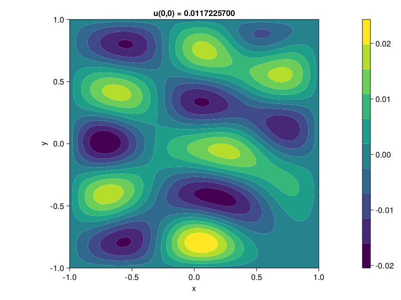
2D Helmholtz#
An important variation on the Poisson equation is the Helmholtz equation, which plays a major role in wave propagation:
where \(k\) is a real parameter. Here is an example solution:
p17: Helmholtz eq.#
N = 24
# Set up spectral grid and tensor product Helmholtz operator:
⊗ = kron
D, x = D, y = cheb(N)
F = [exp(-10 * ((y - 1)^2 + (x - 0.5)^2)) for x in x[2:N], y in y[2:N]]
D² = (D^2)[2:N, 2:N]
k = 9
L = I(N-1) ⊗ D² + D² ⊗ I(N-1) + k^2 * I

# Solve for u, reshape to 2D grid, and plot:
u = L \ vec(F)
U = zeros(N+1, N+1)
U[2:N, 2:N] = reshape(u, N-1, N-1)
xx = yy = -1:1/50:1
UU = gridinterp(U, xx, yy)
value = U[N÷2 + 1, N÷2 + 1]
0.011722570002652808
fig = Figure()
Axis(
    fig[1, 1],
    aspect = DataAspect(), xlabel="x", ylabel="y",
    title = f"u(0,0) = {value:.10f}"
)
co = contourf!(xx, yy, UU)
Colorbar(fig[1,2], co)
fig