2. Step forcing¶

Here is one of our basic building blocks for discontinuous phenomena.

Definition 2.3 (Unit step function)

The unit step function or Heaviside function $H(t)$ is defined to have zero for $t< 0$ and one for $t\ge 0$. That is, if $T$ is any nonnegative constant, then

\[\begin{split} H(t-T) = \begin{cases} 0, & \text{if $t<T$,}\\ 1, & \text{if $t\ge T$.} \end{cases} \end{split}\]

Note

Another common notation for the unit step function is $u(t)$. You will also sometimes see $u_T(t)$ to mean $u(t-T)$.

Note

In this part of the course we will be considering problems with initial condition given at $t=0$. In that context there is really no difference between $H(t)$ and the constant function 1. It’s mostly $H(t-T)$ for $T>0$ that is of interest.

The unit step function represents throwing on an idealized switch, with the value $T$ representing the start time. If we want to use a more general forcing function $f(t)$ that is absent until the start time, we use

\[ f(t-T)H(t-T). \]

This contributes nothing up to time $T$, at which point $f$ begins as though it is starting from time zero.

It can also be useful for a switch that is on for only a limited time.

Definition 2.4 (Window function)

A window function is the function that is one within a given interval and zero outside of it. Specifically, the function

\[ H(t-S) - H(t-T) \]

is equal to 1 for $S\le t < T$ and 0 elsewhere.

Example

Use step functions to express

\[\begin{split} f(t) = \begin{cases} 7, & 0 \le t < 2, \\ \sin(t), & 2 \le t \lt 5, \\ e^t, & t \ge 5. \end{cases} \end{split}\]

2.1. Piecewise constant forcing¶

Here is a key fact about step forcing in a first-order ODE.

Property 2.5 (1st order ODE with step forcing)

If $x(t)$ solves $x'-a(t)x=H(t-T)f(t-T)$, where $a(t)$ and $f(t)$ are continuous, then $x(t)$ is continuous.

Note

While $x(t)$ is continuous, $x'(t)$ is not. The ODE itself tells us that $x'$ has a jump discontinuity at $t=T$.

Consider problems $x'-ax=f(t)$ with $x(0)=x_0$, in which $a$ is constant and the forcing is piecewise constant. That is,

(2.3)¶\[x'-ax = k_1 H(t-T_1) + k_2 H(t-T_2) + \cdots + k_m H(t-T_m),\]

where the subscripted quantities are constants. Returning to our operator notation $\opA[x]=x'-ax$, we can exploit linearity. Define

\[\begin{align*} \opA[x_h] &= 0, \quad x_h(0)=x_0 , \\ \opA[x_1] & = H(t-T_1),\quad x_1(0)=0, \\ & \vdots \\ \opA[x_m] & = H(t-T_m),\quad x_m(0)=0. \\ \end{align*}\]

Then we set

\[ x(t)=x_h(t)+k_1 x_1(t) + \cdots +k_m x_m(t). \]

As a result, $x(0)=x_0+0+\cdots+0=x_0$, so $x$ satisfies the initial condition. Furthermore,

\[\begin{align*} \opA[x] & = \opA[x_h] & + & \, k_1 \opA[x_1] + & \cdots + & \, k_m \opA[x_m] \\ & = 0 & + & \, k_1H(t-T_t) + & \cdots + & \, k_mH(t-T_m), \end{align*}\]

which shows that $x$ solves the original ODE (2.3). This technique of adding together solutions to linear equations is called superposition.

Really there are only two unique subproblems to solve. One of these is the homogeneous case with nonzero initial condition:

\[ \opA[x_h] = 0, \quad x_h(0)=x_0. \]

By now we know the solution here is $x_h(t)=e^{a t}x_0$. The other type of subproblem is

\[ \opA[x_j] = H(t-T_j),\quad x_j(0)=0. \]

For $0\le t \le T_j$ the forcing is zero, so $x_j(t)= 0e^{at}=0$ zero for this interval. Beginning at $T_j$ we have

\[\opA[x_j]=1, \quad x_j(T_j)=0.\]

This can be solved easily using undetermined coefficients or variation of parameters, with the result $x_j(t)=(e^{a (t-T_j)} - 1)/a$ for $t > T_j$. Putting both time intervals together, we get

\[x_j(t) = \frac{1}{a} H(t-T_j)\cdot \bigl(e^{a(t-T_j)} - 1\bigr).\]

Putting all this together, we get a complete formula.

Formula 2.6 (Piecewise constant forcing, 1st order)

The solution of (2.3) is

(2.4)¶\[x(t) = e^{a t}x_0 + \frac{1}{a} \sum_{j=1}^m H(t-T_j)\cdot \bigl(e^{a(t-T_j)} - 1\bigr).\]

Example

Solve $x'-\frac{1}{10}x=w(t)$, $x(0)=-2$, where $w(t)$ is a function that is 5 for $3 < t \le 6$ and zero elsewhere.

Example

Let the serum drug concentration in a patient be $x(t)$. Suppose this is initially zero when an IV is given at a constant rate of 12 units per hour for 30 minutes. An IVP that models this case is

\[x'=-r x + 12 \left[ 1-H(t-0.5) \right], \quad x(0)=0,\]

where $t$ is measured in hours. Solve it to find the concentration of the drug over time.

2.2. Numerical solution¶

MATLAB can handle problems with piecewise constant inputs straightforwardly, if we are not overly concerned with efficiency and high accuracy. The preceding example, for instance, is solved via

step = @(t) double(t>0);
dxdt = @(t,x) 0.1*x + 5*(step(t-3) - step(t-6));
[t,x] = ode23(dxdt,linspace(0,8,401),-2);
plot(t,x)
xlabel('t'), ylabel('x(t)')
title('Window forcing')

ans =

    '9.7.0.1296695 (R2019b) Update 4'

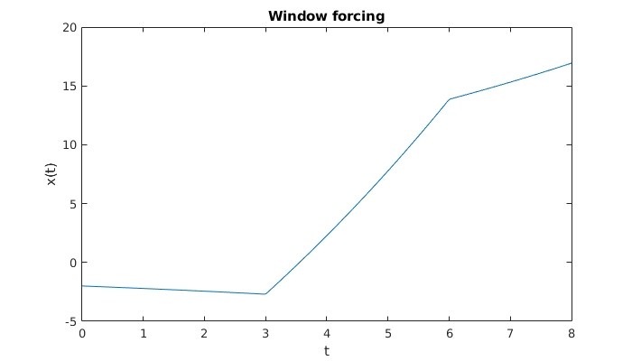
You can clearly see the jumps in $x'(t)$; at $t=3$, the slope increases by 1, and at $t=6$, it decreases by 1.

Notes on linear algebra and ODEs

2. Step forcing¶

2.1. Piecewise constant forcing¶

2.2. Numerical solution¶