4. Convolution¶

4.1. Moving averages¶

The following grabs and plots the closing price of Bitcoin for the last 31 days.

bc = webread('https://api.coindesk.com/v1/bpi/historical/close.json');
data = jsondecode(bc);
v = struct2cell(data.bpi);
v = cat(1,v{:});
plot(v,'-ko')

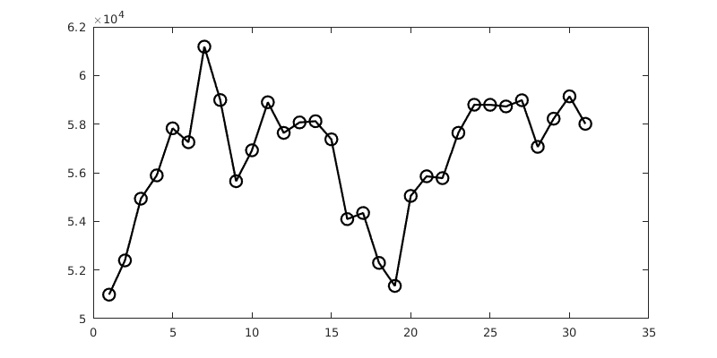
It’s a noisy curve. We can smooth that out by taking 4-day moving averages, for example. There are slick ways to do that, but here is brute force.

plot(v,'-ko')
for i = 4:31
    z(i) = (v(i) + v(i-1) + v(i-2) + v(i-3)) / 4;
end
z(1:3) = NaN;  % not a number
hold on
plot(z)

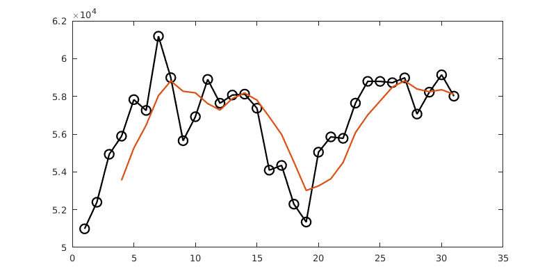
We might decide, however, to weight the most recent values more heavily. Here’s how this might look.

plot(v,'-ko')
w = [4 3 2 1];
for i = 4:31
    z(i) = (w(1)*v(i) + w(2)*v(i-1) + w(3)*v(i-2) + w(4)*v(i-3)) / sum(w);
end
z(1:3) = NaN;  % not a number
hold on
plot(z)

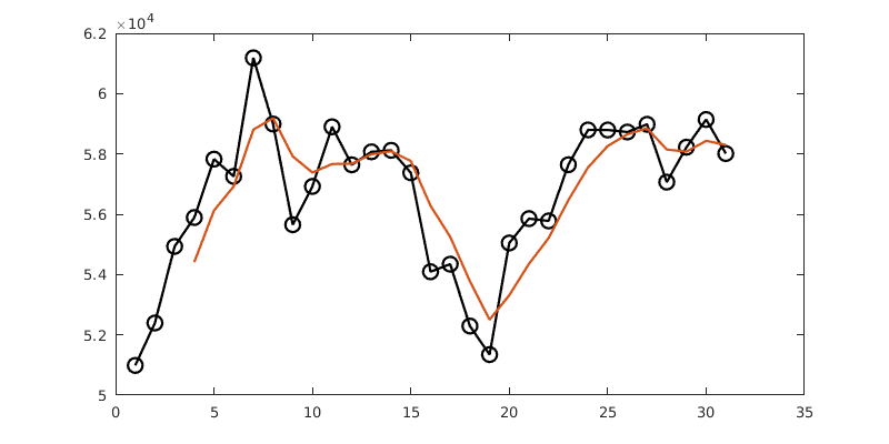
Note that each new value \(z_i\) is a linear combination of the elements of \(v\), weighted by the values in \(w\). And we always go forward 1,2,3,4 in \(w\), while on \(v\) we have a sliding window going backward: \(i,i-1,i-2,i-3\). Put concisely, the indices of \(v\) and \(w\) for each term in the sum add up to \(i+1\), which indexes \(z\).

4.2. Convolution integral¶

The moving average above gave us a certain way to multiply together vectors \(v\) and \(w\) to get a new vector \(z\):

\[z_i = \sum_{j} w_j v_{i-j} \]

(although I reindexed the output vector from \(i+1\) to \(i\) compared to the computer code). This is analogous to a particular way to multiply two functions.

Definition 4.15 (Convolution integral)

\[[f*g](t) = \int_0^t f(t-\tau)g(\tau)\, d\tau\]

This too is a weighted average, with the values of \(g(\tau)\) being multiplied against different windows of the function \(f\) extending backward, such that the arguments of \(f\) and \(g\) sum to \(t\), which is the argument of the result function.

An interesting fact is that while I presented \(f*g\) as \(g\) acting on \(f\), in fact the operation is symmetric:

\[\begin{align*} [g*f](t) & = \int_0^t f(t-\tau)g(\tau)\, d\tau\\ & = \int_t^0 f(u)g(t-u)\, (-du) \\ & = \int_0^t g(t-u)f(u)\, du = [f*g](t) \end{align*}\]

We can also easily prove some other properties we really like to have with multiplication:

Property 4.16 (Convolution)

For functions \(f\), \(g\) and \(h\), all defined for \(t>0\),

\[\begin{align*} f*g &= g*f, \\ f * ( g * h ) &= ( f * g) * h, \\ f * (g+h) &= (f * g)+(f*h),\\ f * 0 &=0, \\ f*\delta &= f, \end{align*}\]

where \(0\) represents the zero function, and \(\delta\) is an impulse.

Note

The last property above may look odd, as we have not discussed impulses in the context of integrals. The property can be confirmed in detail by using the “spike function” \(\delta_\epsilon\) in (3.1) and taking the limit of \(f*\delta_\epsilon\) as \(\epsilon\to 0\).

In particular, if we regard convolution as a sort of multiplication, then the identity element is the impulse \(\delta\).

Warning

It is not true that \(f*1=f\), unless \(f\) is the zero function. A consequence of the next theorem is that the identity for convolution is \(\delta(t)\).

4.3. Convolution theorem¶

Convolution is intimately connected to Laplace transforms.

Theorem 4.17 (Convolution Theorem)

Suppose \(\lx[f] = F(s)\), \(\lx[g] = G(s)\), \(h=f*g\), and \(\lx[h] = H(s)\). Then \(H(s)=F(s)G(s)\).

In words, convolution in time is equivalent to multiplication in transform space.

We now extend some definitions we applied earlier to first-order ODEs.

Definition 4.18 (Impulse response, 2nd order)

Suppose \(\mathcal{A}[x]=x''+bx'+cx\) is a linear, 2nd-order operator. Define \(\delta_\epsilon(t)\) as in (3.1). Let \(x_\epsilon(t)\) be the solution of \(\opA[x]=\delta_\epsilon\), \(x(0)=x'(0)=0\). Then the impulse response of the linear operator is the function

\[\lim_{\epsilon \to 0} x_\epsilon(t).\]

Definition 4.19 (Transfer function, 2nd order)

For the second-order linear operator \(\opA[x]=x''+bx'+cx\) with constants \(b\) and \(c\), the function \(\dfrac{1}{s^2+bs+c}\) is called the transfer function of the operator.

Note

The transfer function is the reciprocal of the characteristic polynomial, and its poles are the characteristic values of the ODE.

All of these ideas come together. The impulse response is the solution of \(\opA[x]=\delta\) with zero initial conditions. Taking transforms gives

\[ s^2 X(s) + b s X(s) + c X(s) = 1, \]

which means that \(X(s)\) is the transfer function.

Theorem 4.20

The impulse response of a linear constant-coefficient equation is the inverse Laplace transform of the transfer function.

Now consider \(\opA[x]=f\), again with zero initial conditions. Transforms imply that

\[ X(s) = \frac{F(s)}{s^2+b s+c} = F(s)G(s), \]

where \(G(s)\) is the transfer function. Thus \(x=f*g\) by the convolution theorem.

Theorem 4.21

The solution \(\opA[x]=f\) with zero initial conditions is the convolution of \(f\) with the impulse response.

Example

Find the general solution of \(x''+36x=\sin(t)\).

In the end, we can avoid Laplace transforms altogether!

The impulse response is equivalent to the solution of \(\opA[x]=0\) with \(x(0)=0\), \(x'(0)=1\), which is a homogeneous problem we can readily solve. Then a particular solution of \(\opA[x]=f\) is only a convolution integral away — although admittedly, the integral might be daunting. It turns out that this process is equivalent to a 2nd-order version of the method of variation of parameters.

For linear problems, all roads lead to the same destination.

Notes on linear algebra and ODEs

4. Convolution¶

4.1. Moving averages¶

4.2. Convolution integral¶

4.3. Convolution theorem¶