5. Direction fields¶

For low-dimensional systems, there is a graphical tool known as a direction field that aids with estimating the behavior of solutions.

5.1. Scalar equations¶

In the scalar equation \(x'=f(t,x)\), \(f\) gives the slope of any solution at any point in the \((t,x)\) plane. Hence, while it is usually not easy to draw solution curves, it is straightforward to draw the instantaneous slopes of them. We give MATLAB code for it here.

function dirfield(varargin)
% DIRFIELD Plot a direction field.
%    DIRFIELD(F,TLIM,XLIM) plots arrows in the (t,x) plane that represent
%    the slope field of the ODE dydt = F(t,y). The function F must accept
%    both arguments. The vectors TLIM and XLIM define the bounds of the 
%    plot in their respective directions.
%
%    DIRFIELD(F,G,XLIM,YLIM) plots arrows in the (x,y) plane that
%    represent the slope field of the ODE system 
% 
%       dx/dt = f(x,y),  dy/dt = g(x,y). 
%
%    Functions F and G must accept (x,y) as arguments. The vectors XLIM and
%    YLIM define the bounds of the plot in their respective directions.
%
%    If an additional input argument is present at the end, the direction
%    vectors are all normalized to have unit length, so speed information
%    is taken out of the picture. This might be better when some arrows
%    would otherwise get too small.
%
%    Examples:
%
%       dirfield(@(t,y) y,[0 3],[-1 1])
%
%       dirfield(@(t,y) t^2-y,[0 2],[-1 1])
%
%       f = @(x,y) 3*x - x*y/2;
%       g = @(x,y) -y + x*y/4;
%       dirfield(f,g,[0 10],[0 12])
%
%    See also QUIVER.

% Copyright 2021 by Toby Driscoll. Free for non-commercial use. 

[f,g] = varargin{1:2};
if isnumeric(g)    % y'=f(t,y)
    xlim = g;
    ylim = varargin{3};
    denorm = (nargin > 3);
    drawfield(@(x,y) 1,f,xlim,ylim,denorm)
    xlabel t, ylabel y
    title(['Slope field for y''=', func2str(f)])

else               % x'=f(x,y), y'=g(x,y)
    [xlim,ylim] = varargin{3:4};
    denorm = (nargin > 4);
    drawfield(f,g,xlim,ylim,denorm)
    xlabel x, ylabel y
    title(['Direction field for x''=',func2str(f),', y''=', func2str(g)])
end
end

function drawfield(dxdt,dydt,xlim,ylim,denorm)

% Set up grid in (x,y) plane 
x = linspace(xlim(1),xlim(2),25);
y = linspace(ylim(1),ylim(2),25);
[X,Y] = meshgrid(x,y);

% This is safer than assuming the user vectorizes the inputs.
U = zeros(size(X));  V = U;
for i = 1:numel(X)
    U(i) = dxdt(X(i),Y(i));  V(i) = dydt(X(i),Y(i));
end

if denorm 
    U = U./sqrt(U.^2+V.^2);  V = V./sqrt(U.^2+V.^2);
end

% Make the plot and pretty it up
quiver(X,Y,U,V)
axis tight

end

For instance, the logistic equation \(x'=ax-bx^2\) can be visualized for \(a=3\), \(b=2\) via

f = @(t,x) 3*x-2*x^2;
dirfield(f,[0 2],[0 1.6])

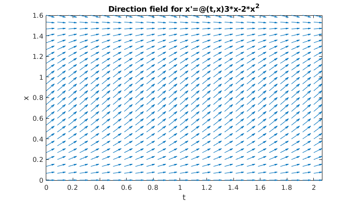
Since the logistic equation is autonomous, the picture is the same along every vertical line. Here you can clearly see the instability of \(\hat{x}=0\) and asymptotic stability of \(\hat{x}=K=1.5\).

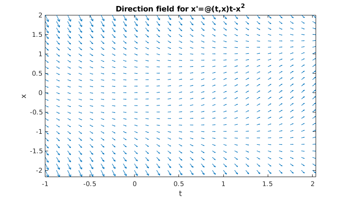
Here is a direction field for \(x'=t-x^2\). Note that the arrows are horizontal along the sideways parabola \(t=x^2\), because that is where the slope is zero.

f = @(t,x) t-x^2;
dirfield(f,[-1 2],[-2 2])

5.2. Autonomous 2D equations¶

An autonomous system in two dimensions has the particular form

\[\begin{align*} \dd{x_1}{t} & = f_1(x_1,x_2), \\ \dd{x_2}{t} & = f_2(x_1,x_2), \\ \end{align*}\]

or, if we prefer to name \(x_1\) and \(x_2\) as \(x\) and \(y\),

\[\begin{align*} \dd{x}{t} & = F(x,y), \\ \dd{y}{t} & = G(x,y). \\ \end{align*}\]

In this case we interpret a solution \([x(t),y(t)]\) as a curve in the \(x-y\) plane parameterized by \(t\). The tangent vector to this curve is

\[ \bigl[ x'(t),y'(t) \bigr] = \bigl[ F(x,y), G(x,y) \bigr]. \]

This quantity can be drawn as a vector field in the \(x-y\) plane, without knowing the solution.

For instance, here is a direction field for the linear ODE system

\[\begin{align*} \dd{x}{t} & = -y,\\ \dd{y}{t} & = x. \end{align*}\]

F = @(x,y) -y;   G = @(x,y) x;
dirfield(F,G,[-2 2],[-2 2])

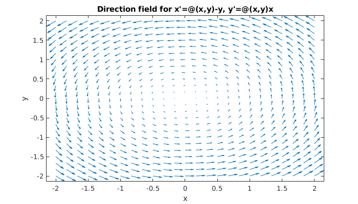
Based on this picture, we should expect to see solutions circulating around the origin. In fact, this system is \(\bfx'=\bfA\bfx\) with matrix \(\bfA=\twomat{0}{-1}{1}{0}\), and the origin is a center.

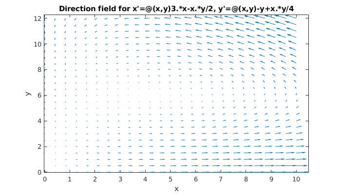
Here is a slope field in the first quadrant for the nonlinear system

\[\begin{align*} \dd{x}{t} & = 3x - \frac{1}{2} x y,\\ \dd{y}{t} & = \frac{1}{4} x y - y. \end{align*}\]

F = @(x,y) 3.*x-x.*y/2;
G = @(x,y) -y + x.*y/4;

dirfield(F,G,[0 10],[0 12])

Notes on linear algebra and ODEs

5. Direction fields¶

5.1. Scalar equations¶

5.2. Autonomous 2D equations¶